The heart of any physics engine is a collision detection system that provides information needed for calculations of the constraint forces. This forces must be calculated to resolve equations that describe the motion of rigid bodies. So, first of all, we need a system that can handle a collision detection in a system of rigid bodies and be able to generate contact information.

Contact detection system has to deal with bodies penetrations and time-zero intersections, because of finite time step and numerical errors. This system must provide information about the contact time and contact position. Generally, there would be a set of intersection points, so there is no a contact point but there is a contact manifold. Let us omit for a while problems of finding exact contact information, assume we need only information if collision happened or not.

How can we detect collisions in a system of interacting objects? If we do not make any special assumptions, we have to consider that all possible bodies pairs potentially can collide. So, in the most naive solution, we have to check all possible pairs of interacting objects. Obviously, this is an extremely expensive approach.

Broad phase.

Actually, not all objects interact with all other objects in the same frame. Moreover, usually, objects interact only with nearest surrounding them objects. So, we can take advantage of the spatial locations of objects to optimize collision detection algorithm. This future of objects distribution in the system is referred to as spatial coherence. For most cases it is possible to assume that dynamic objects do not move significantly between two simulation steps, that is called temporal coherence. Exploiting of spatial and temporal coherence allows culling pairs of objects that definitely can't be in a contact. Usually, objects distribution in space is rather sparse, so the number of real contacts are much less than total possible pairs, that makes collision culling very effective. Such collision culling algorithms are referred to as broad phase algorithms.

Collision detection process can be divided into several phases, typically distinguish next phases:

• Broad phase. The roughest and quick intersection test. The main purpose is to inexpensively eliminate huge amount of collisions.
• Medium phase. More accurate test. The main purpose is to eliminate the rest of potential collisions to reduce the load on final phase.
• Narrow phase. The final phase that performs accurate intersection test and returns all contact properties.

In some cases, there can be only two phase: broad and narrow or medium and narrow, depending on the system properties.

Axis aligned bounding boxes.

Perhaps the most popular approach to cull collisions in broad phase is to use axis aligned bounding boxes (AABB). Each object in the system is represented with appropriate AABB, so that the object is inscribed into the AABB. The AABB is a volume that has a form of a box, sides of that are parallel to the coordinate system planes. If two AABBs are not overlapping, then objects contained by them do not intersect. In the opposite case, objects may intersect and that require more accurate check in the next phase. Overlap test of two AABBs does not depend on the type of objects inscribed in them and much cheaper than any other intersection test between two objects. Another distinguishing feature of AABB is that overlapping detection can be split into independent checks, one for each axis. The image below describes how the checks are performed for 2D space.

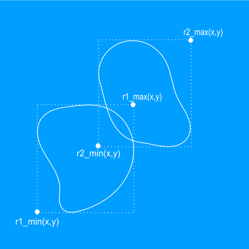Two AABB volumes intersect whenever each of the intervals they occupy on the corresponding axle overlap. This statement in case of 2D problem can be written as:.

The code of function that tests two AABB for overlapping is rather simple:

bool Overlapping(AABB bodyA, AABB bodyB) 
{
  if ((bodyA.xmax < bodyB.xmin) || (bodyA.xmin > bodyB.xmax)) 
  {
    return false; 
  } 
  if ((bodyA.ymax < bodyB.ymin) || (bodyA.ymin > bodyB.ymax)) 
  { 
    return false; 
  } 
  return true; 
}  

Despite the benefit from AABB based culling, we still need to compare all possible pairs of interacting objects to generate the list of potential collisions. Despite the fact that AABB intersection test is extremely cheap, this brute-force approach applicable only for systems with very small amount of interacting objects because it is an O(n²) algorithm. There are several more efficient approaches that use coherence of the objects in the system.

Sweep and prune approach.

I would like to talk about one of these algorithms - sweep and prune (also known as sort and sweep). There is an article on Wikipedia about this approach link.The main idea of this algorithm is based on sorting the intervals that are occupied by the projections of AABBs to the corresponding axle. Let's get a closer look two one dimensional problem first, and then extend the ideas to 2D problem.

Suppose we have a set of intervals that may overlap and that represent an AABBs in one dimension. Each interval formed by two points that are referred to as endpoints. We have already talked about the condition when two intervals overlap, for 1D problem it is as simple as:

Let's sort all our endpoints in ascending order. All endpoints should be market as beginning or ending value. It should be noted that we need to keep track of which endpoints belong to which interval and vice versa. Suppose, we can mark any interval from the set as active or inactive, initially, all intervals are inactive. Next, we iterate over this sorted list and do the following thing:

• Get the endpoint we currently iterating through, figure out what interval contains this endpoint, let's refer to this interval as .
• If a beginning endpoint is encountered then mark appropriate to this endpoint interval active. If there are any other active intervals, all of them are reported as intersecting with the interval.
• If an ending endpoint is encountered then mark the interval as inactive.

Thus, we have two phases: the first one is sorting phase and the second one, we have described, is referred to as sweep phase. This two phases gave one of the names of algorithm: sort and sweep. The time complexity of the sorting phase depends on the type of algorithm it uses, for general case let it be . The complexity of the sweep phase is , since we simply iterate through the list, so total complicity of broad phase would be . That is asymptotically faster than naive approach.

Let's consider sorting phase. We know, that the system of dynamic objects has the property of temporal coherence, that means since we have sorted all endpoint once, at each further step we would have almost sorted list. If objects move only a small distance, then we need to do only a few swaps to make the list sorted again. More over, it should be noted that those endpoints, that are out of order, would be located close to the place of their right order. For this kind of nearly sorted lists, the insertion sort perhaps is the best choice. Despite the fact that for general input it is an algorithm, for nearly sorted data it is , where is the number of swaps occurred. Depending on velocities, sizes and distribution of objects, for the majority of practical cases it is likely that for a better part of frames there wouldn't be a need for swaps at all. Thus under certain conditions, the sweep and prune algorithm would be close to , but generally, it is is an optimal sorting algorithm is used or for the worst case if insertion sort is used.

Producer consumer model.

Let us turn now to the second phase - sweep. As was mentioned above, it's complexity is , but there is still a possibility to optimize it. Due to temporal coherence, the list of overlapping intervals won't differ much from frame to frame. There is no reason to generate the whole list of overlaps every frame, instead, we could track only swaps in the first phase and apply the modifications to the list of overlaps. Let's look at the interaction between these two phases in terms of producer-consumer model. In other words, the sorting phase produces events and the sweep phases consumes them, applying modifications to the overlaps list. What type of events can be produced? Depending on the type of endpoint were swept, three actions are possible:

• No events are produced. The swap does not change the intersection status of intervals.
• An insert event is produced. A new overlapping pair is gained due to the swap.
• A remove event is produced. A pair of overlapping intervals is lost.

To make things clear, let's first look at the listing of insertion sort algorithm written in C++ like pseudocode.

void SortEndpoints(Endpoint* endpoints, int n)
{
	for (int i = 0; i < n; i++)
	{
		Endpoint key = endpoints[i];
		int j = i - 1;
		while (j >= 0 && key < endpoints[j])
		{
			Swap(endpoints[j], endpoints[j + 1]);
			--j;
		}
		endpoints[j + 1] = key;
	}
}

If the key value is less than any of the previous endpoints, then a swap occurs. Comparison of two endpoints we will discuss later, just consider it as a comparison of its coordinate value. How would the swap effect the overlaps list? Let's infer the rules of how the events should be generated.

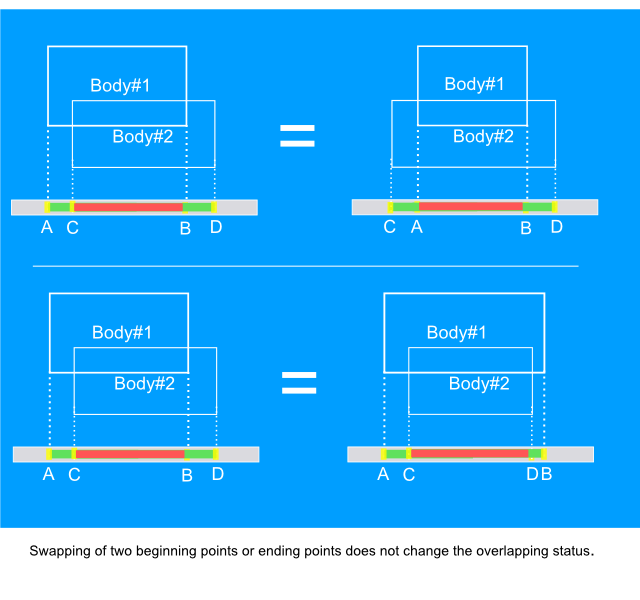
If two beginning or two ending endpoints are swept it is clear that overlapping status won't change. Indeed, if two intervals overlap, they will continue to be overlapped when their beginning endpoints are swept. Completely the same situation occurs when two ending endpoints are swept, the picture below shows both cases.

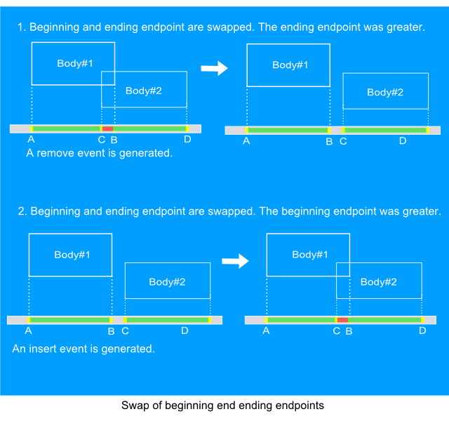
If beginning and ending endpoints are swept then the overlapping status of appropriate intervals is changed. Possible two situations: an intersection is gained and an intersection is lost. Let's assume that the values of the endpoints are sorted in ascending order, then if the beginning endpoint was greater, the overlapping is gained. Alternatively, if the ending endpoint was greater, then the overlapping is lost. The image below describes both situations.

Let's rewrite the pseudo code of insertion sort so that in addition to sorting, it generates insertion/remove events:

void SortEndpoints(Endpoint* endpoints, int n)
{
    for (int i = 0; i < n; i++)
    {
        Endpoint key = endpoints[i];
        int j = i - 1;
        while (j >= 0 && key < endpoints[j])
        {
            Endpoint ep0 = endpoints[j];
            Endpoint ep1 = endpoints[j + 1];
            // ep1 was greater then ep0, but now it is less, 
            // so these endpoints should be swapped.
            if (ep0.IsBeginning())
            {
                if(ep1.IsEnding())
                {
                    // ep1 is ending endpoint, 
                    // so remove event should be generated.
                    PushEvent(ep0.GetIndex(), ep1.GetIndex(), Event::Remove);
                }
            }
            else
            {
                if (ep1.isBeginning())
                {
                    // ep1 is beginning endpoint, 
                    // so insert event should be generated.
                    PushEvent(ep0.GetIndex(), ep1.GetIndex(), Event::Insert);
                }
            }
            Swap(endpoints[j], endpoints[j + 1]);
            --j;
        }
        endpoints[j + 1] = key;
    }
}

When all the events are generated, we need to go through them and apply changes to the overlaps set, as was mention above, this happens in the sweep phase. We will use a set container for the overlaps to be able to quickly insert and remove pairs of intervals. Pseudo code for sweep phase is listed below:

void Sweep(Event* events, int n, set& ovelapsSet)
{
    for(int i = 0; i < n; i++)
    {
        Pair pair(events[i].GetIndex0(), events[i].GetIndex1());
        if (events[i].GetType() == Event::Remove)
        {
            ovelapsSet.erase(pair);
        }
        else
        {
            ovelapsSet.insert(pair);
        }
    }
}

After the overlaps set is updated it can be passed to the narrow phase. There is an insignificant detail about overlap set that I will refer later, the case is that iterating through all the set is not very efficient in comparison with iterating through a simple array.

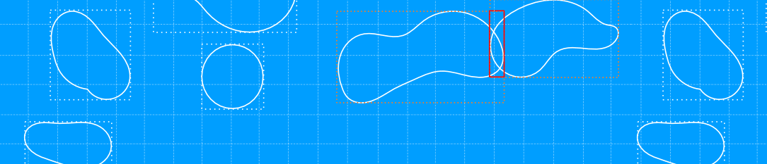
As we can see, nor sort phase neither sweep phase do not generate hole data from scratch every frame, both phases are only updating existing data. This means that sort and sweep algorithm represents an incremental approach, that makes it extremely fast. The gif animation below describes the process on the time interval of several frames. It can be seen, that body#1 moves from the left position to the right one, meanwhile entering and exiting the intersection with the other two bodies. It is remarkable, that the overlapping list is updated only when the states of intersections are changed.

Implementation of the algorithm.

An example application was written, to demonstrate the ideas were described above. The source code of the example you can find at GitHub: BroadPhase. The demonstration application is written in C++ and uses CImg library to visualize the process. This application is a simplified physics engine that demonstrates the basic concepts, particularly a part that runs the broad phase. There are two implementations of broad phase:

• Naive approach.
• Sweep and prune.

You can specify the approach to use at runtime, launch the executable with flag -h for more details.

Below, I would like to describe some details related to the implementation of the sweep and prune approach.

First of all, before we turn to the implementation of the broad phase, let's consider the top-level physics simulation loop. The loop handles the execution of physics engine phases and renders simulated objects to visualize the process. This loop starts just after the initialization of the application and executes until the application is going to close. You can find implementation of this loop in the method Run of the Application class. Perhaps it is not a good idea to call methods that related to the internals of physics engine directly from the application loop, but this way you can see the whole picture at once. The pseudo code that represents this simulation loop is listed below:

// Application run loop
while (!IsGoingToClose())
{
	for (int i = 0; i < SubStepsCount; ++i)
	{
		// Broad Phase
		UpdateAABBList();
		GenerateOverlapList();

		// Narrow phase
		DetectCollisions();

		// Collision response
		ResolveCollisions();
		UpdateObjectsMotion();
	}

	// Draw all bodies
	DrawFrame();
}

From the pseudo code, it can be seen that per each frame draw there are several physical frames, called sub-steps. Count of the sub-steps usually may vary from a single frame to a dozen of frames, depending on how much the system properties vary from frame to frame.

The broad phase is divided into two steps: updating of AABBs list and generating the overlaps list. First, we need to update the AABBs, to make sure that all AABBs contain the bounds of appropriate objects. On the second step, using the updated AABBs list as input, the overlaps list is generated.

We are going to create a class that will hide implementation details of the broad phase. More over, as we want to implement two approaches, we need to create a common interface that will be used as a base class.

Let's declare an interface that will be used to get access to the classes that implements both approaches:

class IBroadPhase
{
public:
	virtual ~IBroadPhase(){};
	virtual void UpdateAABBList(const std::vector bodiesList) = 0;
	virtual const std::vector >& GenerateOverlapList() = 0;
};

Lets refer to the sweep and prune approach. Listing below contains declaration of the class that implements broad phase using sweep and prune algorithm.

class BroadPhaseSS : public IBroadPhase
{
public:
	BroadPhaseSS(int bodiesCount);

	virtual void UpdateAABBList(const std::vector& bodiesList);
	virtual const std::vector >& GenerateOverlapList();

private:
	void UpdateEndPoints();
	void UpdateIntervals(std::vector& endpoints, std::vector& lookUp);
	bool Overlapping(int i0, int i1, const std::vector& lookUp, const std::vector& endpoints);
	
	std::vector m_aabbList;
	std::vector m_endPointsX;
	std::vector m_endPointsY;
	std::vector m_lookUpX;
	std::vector m_lookUpY;
	std::vector m_events;
	std::set > m_ovelapsSet;
	std::vector > m_overlapingList;
};

The method GenerateOverlapList, it is a part of IBroadPhase interface and it encapsulates all the stuff needed to run sweep and prune. Let's write a skeleton of this method in pseudo code:

const std::vector >& BroadPhaseSS::GenerateOverlapList()
{
	UpdateEndPoints();
	UpdateIntervals(m_endPointsX, m_lookUpX);
	UpdateIntervals(m_endPointsY, m_lookUpY);
	Sweep(m_events, m_ovelapsSet);
	m_overlapingList = GenerateOverlapList(m_ovelapsSet);
	return m_overlapingList;
}

The only thing that we didn't talk about is updating of the endpoints values. Because the endpoints are sorted according to their value, we are not able to access them directly. To be able to transfer updated coordinates from the list of aabb to the sorted list of endpoints we need to use a lookup table, that would bind the aabb index with the current position of the endpoint in the sorted list.

Let's get a closer look to the base structures of the sort and sweep algorithm: endpoint and event. The endpoint structure keeps its type (beginning or ending) and the value of coordinate that is related to the axle that endpoint belongs to. In addition, it should contain a reference to the aabb, in other words, the interval, that it is related to (in the simplest case it is an ID, that corresponds to the index of aabb in the array). The endpoint class, that implements all the stuff described above is listed below:

class EndPoint
{
public:
	enum Type
	{
		Minimum,
		Maximum
	};
	void Set(unsigned short aabbIndex, float value, Type type)
	{
		m_aabbIndex = aabbIndex;
		m_value = value;
		m_type = type;
	};

	int GetIndex() const
	{
		return m_aabbIndex;
	}
	;
	Type GetType() const
	{
		return m_type;
	};

	int GetLookUp() const
	{
		return 2 * m_aabbIndex + (m_type == Maximum ? 1 : 0);
	};

	bool operator < (const EndPoint& other) const
	{
		if (m_value == other.m_value)
		{
			return GetType() < other.GetType();
		}
		else
		{
			return m_value < other.m_value;
		}
	};

	float	m_value;
	Type	m_type;
	int	m_aabbIndex;
};

As you can see, there is a method in event class, that we didn't mention - GetLookUp(). The purpose of this method is to get the index of the endpoint in given lookup table. For more details, it is better to refer to the source code that can be found in the GitHub repository.

The event structure should keep information about its type and indices of the overlapping intervals.

class Event
{
public:
	enum Type
	{
		Remove,
		Insert
	};
	
	Event()
	{};
	
	Event(int index0, int index1, Type type)
	{
		m_index0 = index0;
		m_index1 = index1;
		m_type = type;
	};
	
	Type GetType() const
	{
		return m_type;
	};
	
	int GetIndex0() const
	{
		return m_index0;
	};
	
	int GetIndex1() const
	{
		return m_index1;
	};
	
	Type m_type;
	int m_index0;
	int m_index1;
};

Comparison of the approaches.

The scene, that was chosen for the simulation, corresponds to the worst case scenario. In the most of real world examples the amount of movements made by the objects would be much less. One of the simulation frames is shown below:

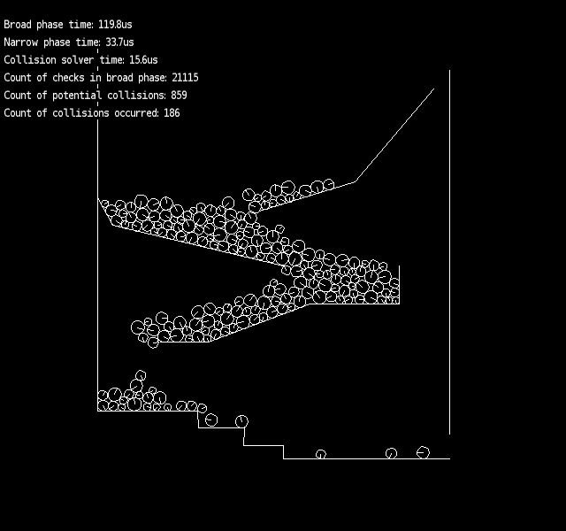
A comparation of the naive and sweep and prune approaches was made for this particular simulation case. The simulation was run on Core i5-4440 @3.10GHz using MSVC 12.0.

The comparison results are plotted below:

There are three curves on the plot. The blue one corresponds to the nave approach while the red one corresponds to the sweep and prune approach. Remaining yellow curve corresponds to the optimized version of the sweep and prune approach. All of the optimizations have a technical nature, not algorithmic. You can find the optimized version at the branch called "Optimized", link.

Let's have a look at the exponent value of the relation of objects count to the broad phase run time. For the range of object count from 50 to 250, the exponent of naive approach is close to 1.8, while for the sweep and prune approach it is close to 1.0 - 1.2. After the count of objects exceeds the value of 300, the exponent of sweep and prune approach begin to grow.

The absolute value of broad phase time run of sweep and prune approach in optimized version is more than ten times faster than the naive approach on the wide range of the number of objects.

It should be noted, that for objects count less than 15, the naive approach has shown a better time run than the sweep and prune approach. So, if the simulation involves less than a couple of dozens of objects, perhaps it is better to use a simple naive approach.