Finite element method allows solving a large variety of engineering and mathematical physics problems. Historically, the first application of FEM was in mechanics, that affected its terminology and first interpretations. Indeed, the essence of the method can be described as follow: the continuous medium is replaced by the equivalent hinged system, that allows representing the system as a statically indeterminate. Solving statically indeterminate hinged rods system is a straightforward and well-known problem. This simplified treatment contributed to the widespread of the method, while strictly speaking this treatment is incorrect. Precise mathematical handling of the method was developed much later of first successful method applications, but it enabled extension of the method to a wide range of problems, not only mechanical.

Today we have a such complex FEM software as ANSYS, Abaqus, Patran, Cosmos, etc. These software packages enable solving structural mechanic, fluid mechanic, thermodynamic, electromagnetic and other problems. Any application that uses FEM approach is believed to be a very complex, sophisticated software.

Here I want to show, that nowadays, using latest tools, writing FEM solver from scratch for two-dimensional flat stress problem is not such big deal. I've selected this kind of problem, because, two-dimensional elastic problems were the first successful examples of the application of FEM. I'm going to use three nodes, liner, triangle element, as it eliminates the need for numerical integration, as it will be shown below.

I'm not going to describe the method in details, here is a lot of literature about it. Instead of this I will concentrate on method implementation and assume that the reader has some basic knowledge of the method. I will try to keep things as simple as possible and give preference to shortness over many programming principles. It is not a tutorial on writing good, maintainable and robust code, but it is a tutorial on implementing FEM approach. So there will be a lot of simplifications, just to concentrate on main goals. If you are interested in, write in comments and I'll post another article with detailed description on how it should be written in terms of good architecture and API design.

Input data

Before proceeding to the method itself, let's find out what type of data will be given to the program as input. The considered body should be split to a large number of small regions, in our case - triangles. So, the continuous medium is replaced by a set of nodes and triangle elements that form a mesh. On the picture below, a simple mesh is shown with corresponding nodes and elements.

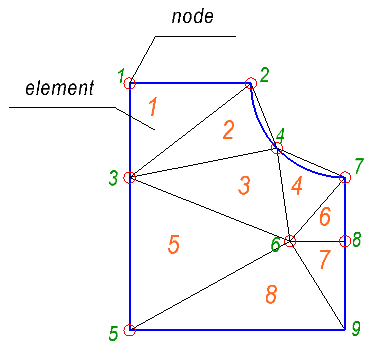
On the picture, nine nodes and eight elements are shown. To describe the mesh, it is needed two lists. The first one, is a list of nodes, that specifies coordinates of each node. The second one is a list of elements. In this list, each element is defined by set of node indices, that forms the element. For our case, we have only triangle elements, so we would have precisely three node indices per element. For example, for the shown above mesh, we would have the following lists:

Nodes list:

0.000000 	31.500000
15.516667 	31.500000
0.000000 	19.489759
18.804134 	23.248226
0.000000 	0.000000
20.479981 	11.365822
27.516667 	19.500000
27.516667 	11.365822
27.516667 	0.000000

Elements list:

1 3 2
2 3 4
4 6 7
4 3 6
7 6 8
3 5 6
6 5 9
6 9 8

It worth to note, that there are multiple ways to do define the same element. The element can be defined by the node indices written clockwise or counterclockwise. Commonly used only counterclockwise notation, so we would assume that all elements are defined that way.

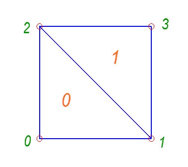
Let's create some input file with a full description of the problem. First of all, to make things simpler, it's better to use indexing that starts from zero, not from 1, because in C/C++ languages array indexing is from zero. It is not something that should be done only that way and not the other. There is no problem in using indexing starting from 1, we will use indexing starting from zero just to avoid confusion. For the first input file, it is better to create the simplest mesh ever possible. So let's create the following mesh:

Let the first line be a description of material properties. For example, for the steel, with Poisson's ratio and Young's modulus :

0.3 2000

Then, follows a line with count of nodes and then lines with the nodes list:

4
0.0 0.0
1.0 0.0
0.0 1.0
1.0 1.0

Then, follows a line with elements count and then lines with the elements list:

2
0 1 2
1 3 2

Next, we will specify constraints. Constraints apply restriction on node movements. It should be understood as we explicitly set one or two components of deflection at specific node to zero (or any fixed value in general). So, we need a list of node, with specified restrictions. The type of restriction will be specified with a number: 1 – forbidden deflection in X direction, 2 – forbidden deflection in Y direction, 3 – forbidden deflection in both, X and Y directions. The first line specifies the count of constraints:

2
0 3
1 2

Then, we need to specify loads. Here we would work only with nodal loads. To be precise, nodal loads should not be treated as a load in general sense. I’ll cover this aspect later, but know let’s think about them just as about loads at node. We need a list with node indices and corresponding force vector. The first line specifies the count of forces applied:

2
2 0.0 1.0
3 0.0 1.0

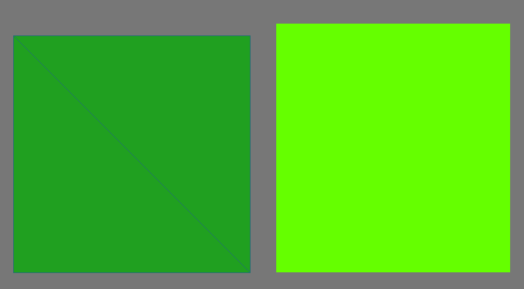
It can be easily seen, that we have a square body, that has constraints at its bottom and it is stretched with force applied at its top. Here is the whole input file:

0.3 2000
4
0.0 0.0
1.0 0.0
0.0 1.0
1.0 1.0
2
0 1 2
1 3 2
2
0 3
1 2
2
2 0.0 1.0
3 0.0 1.0

Eigen – math library

Before starting writing code, I want to introduce a great math library – Eigen eigen.tuxfamily.org. It is a mature, robust and effective library that has extremely clean and expressive C++ API. It does a lot of optimizations at compile time due to the template meta-programming and able to perform explicit vectorization using SSE 2/3/4, ARM NEON instruction sets that result in extremely fast code. As for me, this library is great because it enables to allows to write complex math calculations in short and expressive way.
Before we continue, let me make some introduction to some of Eigen API that we will use later.

There are to types of Matrices: dense and sparse. We will use both of them. In case of dense matrix, all the elements are kept in plane way in memory. This type of matrices is good for relatively small matrices or matrices with small amount of zero elements. Spare matrices are good for storing large, sparse matrices with small amount of non zero elements. We will use sparse matrix for global stiffness matrix.

Dense matrices

To use dense matrices you will need to include header . There are two main types of dense matrices: fixed size and dynamic size. Fixed sized matrix it is a such matrix, that size is known at compile time. Dynamic size matrix, it is a such matrix, that size is not known at compile time and memory for this matrix should be allocated at compile time. The fixed size matrices should be preferred, whenever it possible, because dynamic size matrices cause heap memory allocations and restricts optimizations that compiler can do. Fixed size matrices can be allocated on stack and compiler may expand loops and do some more optimizations, as it knows the exact size at compile time. It worth to note, that the mixed type is also possible, when matrix has fixed count of rows, but dynamic count of columns or vice versa.

Fixed size matrix can be defined in the following way:

Eigen::Matrix m;

Where m is a fixed size 3×3 matrix pf floats. You may also use the following predefined types:

• Eigen::Matrix2i

• Eigen::Matrix3i

• Eigen::Matrix4i

• Eigen::Matrix2f

• Eigen::Matrix3f

• Eigen::Matrix4f

• Eigen::Matrix2d

• Eigen::Matrix3d

• Eigen::Matrix4d

There are a bit more predefined types, these are the basic ones. The digit denotes the dimension of square matrix and the letter denotes type of element. i – integer, f – float, d – double.

Vectors are just the same matrices. You may define a column vector as follows:

Eigen::Matrix v;

Or you may use one of predefined types (notation is the same as for matrices):

• Eigen::Vector2i

• Eigen::Vector3i

• Eigen::Vector4i

• Eigen::Vector2f

• Eigen::Vector3f

• Eigen::Vector4f

• Eigen::Vector2d

• Eigen::Vector3d

• Eigen::Vector4d

As a quick introduction, I have written the following self-descriptive example:

#include <Eigen/Dense>
#include <iostream>

int main()
{
	//Fixed size 3x3 matrix of floats
	Eigen::Matrix3f A;
	A <<	1, 0, 1,
			2, 5, 0,
			1, 1, 2;

	std::cout	<< "Matrix A:" 
				<< std::endl
				<< A 
				<< std::endl;

	//Access to matrix element [1, 1]:
	std::cout	<< "A[1, 1]:"
				<< std::endl
				<< A(1, 1) 
				<< std::endl;

	//Fixed size 3 vector of floats
	Eigen::Vector3f B;
	B << 1, 0, 1;

	std::cout	<< "Vector B:"
				<< std::endl
				<< B
				<< std::endl;
	
	//Access to vector element [1]:
	std::cout	<< "B[1]:"
				<< std::endl
				<< B(1)
				<< std::endl;

	//Multiplication of vector and matrix
	Eigen::Vector3f C = A * B;
	std::cout	<< "C = A * B:"
				<< std::endl
				<< C
				<< std::endl;
	
	//Dynamic size matrix of floats
	Eigen::MatrixXf D;
	D.resize(3, 3);

	//Let matrix D be an identity matrix:
	D.setIdentity();

	std::cout	<< "Matrix D:" 
				<< std::endl
				<< D
				<< std::endl;

	//Multiplication of matrix and matrix
	Eigen::MatrixXf E = A * D;
	std::cout	<< "E = A * D:" 
				<< std::endl
				<< E
				<< std::endl;

	return 0;
}

The output:

Matrix A:
1 0 1
2 5 0
1 1 2
A[1, 1]:
5
Vector B:
1
0
1
B[1]:
0
C = A * B:
2
2
3
Matrix D:
1 0 0
0 1 0
0 0 1
E = A * D:
1 0 1
2 5 0
1 1 2

For more information check the documentation of Eigen: eigen.tuxfamily.org/dox/GettingStarted.html

Sparse matrices

Sparse matrix is a bit more complicated type of matrix. The main idea is not to store the whole matrix in a plain way in the memory but store only non-zero elements. It is a quite common case in engineering when a large matrix has very few non-zero elements. When assembling global stiffness matrix of a fem model, the count of the non-zero elements can be less than 0.1% of all elements. It is not a big deal for modern FEM packages to solve problems with hundred thousands of nodes, more over, these problems may be solved on a regular hardware. If we try to allocate place to store the global stiffness matrix in a plane way, we will face the following problem:

The size of memory needed to store the dense matrix is extremely large! The sparse matrix would need 10,000 times less amount of memory.

Sparse matrices use memory much more efficiently, as only non-zero elements are kept. Sparse matrices can be represented in two ways: compressed and uncompressed. In the uncompressed mode, it is easy to add or remove an element from the matrix but is not optimal in terms of memory use. Eigen is able to convert a uncompressed matrix to compressed form very easily, more over it does it transparently, you won't have to do it explicitly. Most of the algorithms require a compressed matrix, and applying any of these algorithms will convert the matrix to compressed mode. And vice versa, adding/removing element will convert matrix to uncompressed mode.

How can we construct matrix? A good way to do it is to use so called Triplets. It is a data structure, moreover, it is a template class, that represents a single element and its position in the matrix. We can construct a sparse matrix directly from a vector of triplets.

For example, let's say we have the following sparse matrix:

0	3	0	0	0
22	0	0	0	0
0	5	0	1	0
0	0	0	0	0
0	0	14	0	8

The first thing we need to do, is to include an appropriate header of Eigen library: . Then we construct an empty sparse matrix of dimension 5x5.
Next, we define a vector of triplets and fill it with values. The constructor of triplet accepts arguments as follows: i, j, value.

#include <Eigen/Sparse>
#include <iostream>

int main()
{
	Eigen::SparseMatrix<int> A(5, 5);

	std::vector< Eigen::Triplet<int> > triplets;

	triplets.push_back(Eigen::Triplet<int>(0, 1, 3));
	triplets.push_back(Eigen::Triplet<int>(1, 0, 22));
	triplets.push_back(Eigen::Triplet<int>(2, 1, 5));
	triplets.push_back(Eigen::Triplet<int>(2, 3, 1));
	triplets.push_back(Eigen::Triplet<int>(4, 2, 14));
	triplets.push_back(Eigen::Triplet<int>(4, 4, 8));

	A.setFromTriplets(triplets.begin(), triplets.end());

	A.insert(0, 0);
	std::cout << A;

	A.makeCompressed();

	std::cout << std::endl << A;
}

The output will be as follows:

Nonzero entries:
(0,0) (22,1) (_,_) (3,0) (5,2) (_,_) (_,_) (14,4) (_,_) (_,_) (1,2) (_,_) (_,_) (8,4) (_,_) (_,_)

Outer pointers:
0 3 7 10 13  $
Inner non zeros:
2 2 1 1 1  $

0 3 0 0 0
22 0 0 0 0
0 5 0 1 0
0 0 0 0 0
0 0 14 0 8

Nonzero entries:
(0,0) (22,1) (3,0) (5,2) (14,4) (1,2) (8,4)

Outer pointers:
0 2 4 5 6  $

0 3 0 0 0
22 0 0 0 0
0 5 0 1 0
0 0 0 0 0
0 0 14 0 8

Basic data structures

To store the data, we are going to read from the input file, we need to special data structure. Data structure of finite element is shown below. It consists of array of three elements that store Ids of the nodes, that form the finite element. There is also a 3x6 matrix , so called gradient matrix, we will return to it later. The method CalculateStiffnessMatrix will be covered also later.

struct Element
{
	void CalculateStiffnessMatrix(const Eigen::Matrix3f& D, std::vector >& triplets);

	Eigen::Matrix B;
	int nodesIds[3];
};

And one more simple structure, to store data about constraints. It simply consists of enumerated type that defines constraint type and integer value that defines constrained node id.

struct Constraint
{
	enum Type
	{
		UX = 1 << 0,
		UY = 1 << 1,
		UXY = UX | UY
	};
	int node;
	Type type;
};

To keep things simple, we are going to define some global variables. This is always a bad idea to have any global objects, but for this example it is fine. We will need later the following global variables:

• Amount of nodes
• A vector that, define x-coordinate of all nodes
• A vector that, define y-coordinate of all nodes
• A vector of elements
• A vector of constraints
• A vector of loads

In code, we will define them as follows:

int							nodesCount;
int							loadsCount;
Eigen::VectorXf				nodesX;
Eigen::VectorXf				nodesY;
Eigen::VectorXf				loads;
std::vector< Element >		elements;
std::vector< Constraint >	constraints;

Reading input

Before reading something, we need to know from what file to read and where to write output. In the beginning of main function let's check a number of input arguments, note that the first argument is always a path to the executable. So we need three arguments, the second one is a path to the input file, and the third one is a path to the output one. To work with file i/o, for the particular case, file streams from the c++ standard library are very handy. So, we create to file streams, for input and output.

int main(int argc, char *argv[])
{
	if ( argc != 3 )
    {
        std::cout << "usage: " << argv[0] << "  
\n";
        return 1;
    }
		
	std::ifstream infile(argv[1]);
	std::ofstream outfile(argv[2]);

The first line of the input file is material properties, the following lines shows how to read them:

	float poissonRatio, youngModulus;
	infile >> poissonRatio >> youngModulus;

That is it, so simple! This is enough to construct elasticity matrix of isotropic material for the flat stress strain problem, that is defined as follows:

Where did this relation come from? It comes from the Hooke's law, indeed we can obtain the matrix from the following relations:

It worth to note, that flat stress problem means, that the equals to zero, but not the . This set of 2d problems is good for various applications, where considered some flat structures and all forces are acting in plane. There is nothing stopping structure from deforming in direction of normal to the plane, that is why in general not zero. It does not appear in equation above, but can be easily obtained from: , as equals to zero.

Let's construct elasticity matrix using Eigen:

	Eigen::Matrix3f D;
	D <<
		1.0f,			poissonRatio,	0.0f,
		poissonRatio,	1.0,			0.0f,
		0.0f,			0.0f,			(1.0f - poissonRatio) / 2.0f;

	D *= youngModulus / (1.0f - pow(poissonRatio, 2.0f));

Next, we need to read node coordinates. First we read count of nodes, then resize the dynamic vectors for and coordinates. Next, we simply read node coordinates in loop, line by line.

	infile >> nodesCount;
	nodesX.resize(nodesCount);
	nodesY.resize(nodesCount);

	for (int i = 0; i < nodesCount; ++i)
	{
		infile >> nodesX[i] >> nodesY[i];
	}

Next, we need to read elements information. Here we read count of elements, and then ids of nodes for each element:

	int elementCount;
	infile >> elementCount;

	for (int i = 0; i < elementCount; ++i)
	{
		Element element;
		infile >> element.nodesIds[0] >> element.nodesIds[1] >> element.nodesIds[2];
		elements.push_back(element);
	}

Next, we need to read constraint information. Totally the same thing:

	int constraintCount;
	infile >> constraintCount;

	for (int i = 0; i < constraintCount; ++i)
	{
		Constraint constraint;
		int type;
		infile >> constraint.node >> type;
		constraint.type = static_cast(type);
		constraints.push_back(constraint);
	}

You may notice a static_cast, that is needed to transform integer type to constraint type, that we defined in constraint structure earlier.

Next, we need to read loads information. There is one specialty, we create a zero load vector of a size of double nodesCount that represents load at each node, and then fill it with values. The reason, why we do so, will be covered a bit later. The following picture illustrates this load vector:

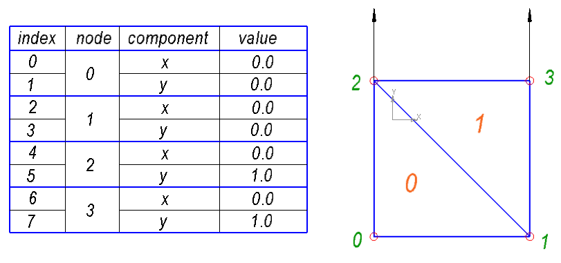
So, for each node, we have two elements in the load vector, that represent and component of load. Thus, x-component of load at some specific node will be stored in element and y-component of load at some specific node will be stored in element .

First, we set the size of load vector twice bigger than the count of nodes. Next, we set all elements to zero. Then we read count of loads. Next, we read all the loads line by line and put the values in corresponding elements of vector.

	int loadsCount;
	loads.resize(2 * nodesCount);
	loads.setZero();

	infile >> loadsCount;

	for (int i = 0; i < loadsCount; ++i)
	{
		int node;
		float x, y;
		infile >> node >> x >> y;
		loads[2 * node + 0] = x;
		loads[2 * node + 1] = y;
	}

Calculating global stiffness matrix

We consider geometrically linear system, with infinitely small deflections. More over, we assume, that the strain is a linear function of stress (Hooke's law). From the basis of structural mechanics, it can be shown, that displacement of each node is a linear function of applied forces. Thus, we can say, that we have the following system of linear equations:

Where: - stiffness matrix; - vector of displacements; - vector of loads, that is vector of external forces. This system of linear equations is often called ensemble, as it represents composition of stiffness matrices of each element, as it will be shown below.

Vector of displacement, for 2d problem can be defined as follows:

Where: and are component and component of displacement at -th node.

And vector of external forces:

Where: and are component and component of external force at -th node.

As we can see, each entry of displacement vector and load vector is a 2-d vector. Instead of this, we can define these vectors as follows:

That is actually totally the same thing, but it simplifies representing of these vectors in code. That is the explanation, why we have created load vector in this way earlier.

How can we construct the stiffness matrix? The essence of global stiffness matrix is a composition of stiffness matrices of each element. If we consider a single element, we can define the same relationship between node displacements and nodal forces. For example for 3-node element:

Where: - stiffness matrix of e-th element; - vector of displacements of e-th element nodes; - vector of e-th element nodal forces ; - indices of element nodes.

What will happen, if one node is shared between two elements? First of all, as far as we treat it as one node, it has the same displacement for all elements, that it forms. The second important consequence is that if we sum nodal forces from each element at this node, the result would be equal to the external force, in other words - load.

The sum of nodal forces at every node equals to the sum of external forces at that node just from the principle of equilibrium. This thing is a bit tricky, because it is not a precise mathematical treatment, but only a handy representation. That is because nodal force is a quite abstract thing, that con not be considered just as a regular force. However this principle is true, but actually is not that simple.

If we sum all the equations for each node, the nodal forces will go. On the right side will be only external forces - loads. So, considering this fact, we can write:

The following picture illustrates the statement above:

To construct the global stiffness matrix, we will create a vector of triplets, and ask every element to fill it with values its stiffness matrix:

std::vector > triplets;
for (std::vector::iterator it = elements.begin(); it != elements.end(); ++it)
{
	it->CalculateStiffnessMatrix(D, triplets);
}

Where std::vector > triplets - vector of triplets, CalculateStiffnessMatrix method of element class, that pushes values of element matrix to triplet vector.

As we have seen before, we can construct the sparse matrix from the vector of triplets:

Eigen::SparseMatrix globalK(2 * nodesCount, 2 * nodesCount);
globalK.setFromTriplets(triplets.begin(), triplets.end());

We do not need to bother about summing values of the same elements of matrix, setFromTriplets method does it automatically.

Calculating element stiffness matrix

We know how to assemble global stiffness matrix from matrices of elements, now we are going see how to construct stiffness matrix of element.
Let's start from interpolating of displacements in the element basing on displacements of its nodes. If displacements of nodes are given, then displacement in any point of element can be obtained by the following equation:

Where [N] is a matrix of functions of position (x, y). These functions are called shape functions. Each component of displacement, u and v can be interpolated dependently, and for the case of three-node element the equation above can be rewritten in the following form:

Or we can wtite the same thing in separate form:

How can a function be interpolated? For simplicity, let's take a scalar field. For three-node linear element, interpolation is linear. To interpolate function, we need to find an equation of the following form:

If the values of f at the nodes are known, then we can write a system of three equations:

Or in matrix form:

From these system of equations we can find unknown vector of values of a:

Let's denote . The interpolation equation finally will be:

Returning to displacements, we can say that:

So, the shape functions will be:

From the field of displacement, we can find field of deformations, using the following well know relation:

Now, we can substitute for u and v, the interpolation formulas obtained earlier:

Or we can write the same thing in a combined form:

Matrix on the right side is usually denoted as matrix B, so we have:

As we have mentioned earlier, the relation between stress and deformation can be written with help of elasticity matrix D:

So, we can substitute the relation for deformations:

To find matrix B, we need to find all partial derivatives of shape functions:

For our particular case of linear element, we see that partial derivatives of shape functions actually are constant, that will save us lot's of time. Multiplying the vector by the inverse C matrix we can obtain:

At this point we see that we have everything to calculate B matrix. To calculate the C matrix we need vectors of position of element nodes, that we can obtain from nodes indices:

Eigen::Vector3f x, y;
x << nodesX[nodesIds[0]], nodesX[nodesIds[1]], nodesX[nodesIds[2]];
y << nodesY[nodesIds[0]], nodesY[nodesIds[1]], nodesY[nodesIds[2]];

Then, we can construct a matrix from three rows:

Eigen::Matrix3f C;
C << Eigen::Vector3f(1.0f, 1.0f, 1.0f), x, y;

Then we calculate inverse matrix of matrix C and assemble B matrix:

Eigen::Matrix3f IC = C.inverse();
for (int i = 0; i < 3; i++)
{
	B(0, 2 * i + 0) = IC(1, i);
	B(0, 2 * i + 1) = 0.0f;
	B(1, 2 * i + 0) = 0.0f;
	B(1, 2 * i + 1) = IC(2, i);
	B(2, 2 * i + 0) = IC(2, i);
	B(2, 2 * i + 1) = IC(1, i);
}

To obtain the stiffness matrix, we need to turn to virtual work. Let's say we have some virtual displacements at nodes of elements:

Virtual displacements should be treated as any infinitesimal displacements that can happen. In a particular problem, we know that only one solution exists and only one set of displacements can take place, but here we consider the element in separate from the problem and trying to figure out what will happen if we apply any displacements. These displacements are called virtual, because they are speculative.

For these virtual displacements, the virtual work of nodal forces will be:

The virtual work of internal stresses in a unit volume for the same virtual displacement:

Or

Substituting the equation for stresses, we can finally obtain:

From the energy conservation law, the virtual work of external forces should be equal to the sum of work of internal stresses over the element volume :

As this relation should be true for any virtual displacement, we can divide the both side of equation by the virtual displacement:

Nodal displacements were taken outside the integral, as they are constant. Now we can see, that the integral is a coefficient of proportionality between the nodal displacements and nodal forces, that means that it is element stiffness:

For the linear element, as we obtained earlier, the matrix B is constant. If material properties are constant too, then the integral became trivial:

Where A - area of element, t - thickness of element. From the properties of triangle, its area can be obtained as half of determinant of matrix C:

Eventually, the code that calculates the stiffness matrix will be:

Eigen::Matrix K = B.transpose() * D * B * C.determinant() / 2.0f;

And the whole method CalculateStiffnessMatrix of element class:

void Element::CalculateStiffnessMatrix(const Eigen::Matrix3f& D, std::vector >& triplets)
{
	Eigen::Vector3f x, y;
	x << nodesX[nodesIds[0]], nodesX[nodesIds[1]], nodesX[nodesIds[2]];
	y << nodesY[nodesIds[0]], nodesY[nodesIds[1]], nodesY[nodesIds[2]];
	
	Eigen::Matrix3f C;
	C << Eigen::Vector3f(1.0f, 1.0f, 1.0f), x, y;
	
	Eigen::Matrix3f IC = C.inverse();

	for (int i = 0; i < 3; i++)
	{
		B(0, 2 * i + 0) = IC(1, i);
		B(0, 2 * i + 1) = 0.0f;
		B(1, 2 * i + 0) = 0.0f;
		B(1, 2 * i + 1) = IC(2, i);
		B(2, 2 * i + 0) = IC(2, i);
		B(2, 2 * i + 1) = IC(1, i);
	}
	Eigen::Matrix K = B.transpose() * D * B * C.determinant() / 2.0f;

	for (int i = 0; i < 3; i++)
	{
		for (int j = 0; j < 3; j++)
		{
			Eigen::Triplet trplt11(2 * nodesIds[i] + 0, 2 * nodesIds[j] + 0, K(2 * i + 0, 2 * j + 0));
			Eigen::Triplet trplt12(2 * nodesIds[i] + 0, 2 * nodesIds[j] + 1, K(2 * i + 0, 2 * j + 1));
			Eigen::Triplet trplt21(2 * nodesIds[i] + 1, 2 * nodesIds[j] + 0, K(2 * i + 1, 2 * j + 0));
			Eigen::Triplet trplt22(2 * nodesIds[i] + 1, 2 * nodesIds[j] + 1, K(2 * i + 1, 2 * j + 1));

			triplets.push_back(trplt11);
			triplets.push_back(trplt12);
			triplets.push_back(trplt21);
			triplets.push_back(trplt22);
		}
	}
}

At the end of the method triples are constructed. They are nothing but values of element stiffness matrix with corresponding indices in global stiffness matrix.

Applying constraints

The obtained system of linear equations can not be solved until the displacement constraints are applied. Displacement of some nodes should be set to zero or some constant value, otherwise the mechanical system will be in motion and the linear system of equation will have rank less than the number of nodes.
As a simplest case, let's consider only setting displacement of constrained nodes to zero. Actually this means remove of some equations from the system. But changing of the number of equation in the system on fly is not trivial to program. Instead of this, the following trick can be applied.

Let's say we have the following system of equations:

To constrain the node, the corresponding element of the matrix should be set to 1, and all elements in that row and column should be set to zero. There should not be any external forces acting on the constrained node in constrained direction. The equation with this node will explicitly give zero displacement for that node, and zeros in the corresponding column will eliminate that displacement from other equations. Let's say we want to constrained displacement along the x axis of the first, and displacement along the y axis of the second node:

To perform this operation, first the indices to be constrained should be determined. To do this, we iterate through the list of constrains and push indexes regarding the type of constrain. Then we iterate through all elements of stiffness matrix and call function SetConstraints. Below the fuction ApplyConstraints is listed:

void ApplyConstraints(Eigen::SparseMatrix& K, const std::vector& constraints)
{
	std::vector indicesToConstraint;

	for (std::vector::const_iterator it = constraints.begin(); it != constraints.end(); ++it)
	{
		if (it->type & Constraint::UX)
		{
			indicesToConstraint.push_back(2 * it->node + 0);
		}
		if (it->type & Constraint::UY)
		{
			indicesToConstraint.push_back(2 * it->node + 1);
		}
	}

	for (int k = 0; k < K.outerSize(); ++k)
	{
		for (Eigen::SparseMatrix::InnerIterator it(K, k); it; ++it)
		{
			for (std::vector::iterator idit = indicesToConstraint.begin(); idit != indicesToConstraint.end(); ++idit)
			{
				SetConstraints(it, *idit);
			}
		}
	}
}

The function SetConstraints checks if the element of the stiffness matrix is in the row or column of constrained node, and if it is, then it sets it to zero or to 1 depending on whether the element is in diagonal or not:

void SetConstraints(Eigen::SparseMatrix::InnerIterator& it, int index)
{
	if (it.row() == index || it.col() == index)
	{
		it.valueRef() = it.row() == it.col() ? 1.0f : 0.0f;
	}
}

To apply constraints the function ApplyConstraints is called:

	ApplyConstraints(globalK, constraints);

Solving and generating output

Eigen library has various solvers for sparse linear equation, we are going to use SimplicialLDLT that is fast direct solver. For demonstration purposes, we will output the initial stiffness matrix and load vector and then output the resulting vector of displacements. Using of the equation solver is quite straightforward and should be clear from the following listing:

	std::cout << "Global stiffness matrix:\n";
	std::cout << static_cast >& > (globalK) << std::endl;

	std::cout << "Loads vector:" << std::endl << loads << std::endl << std::endl;

	Eigen::SimplicialLDLT > solver(globalK);

	Eigen::VectorXf displacements = solver.solve(loads);

	std::cout << "Displacements vector:" << std::endl << displacements << std::endl;

	outfile << displacements << std::endl;

Analyzing output

	std::cout << "Stresses:" << std::endl;

	for (std::vector::iterator it = elements.begin(); it != elements.end(); ++it)
	{
		Eigen::Matrix delta;
		delta << displacements.segment<2>(2 * it->nodesIds[0]),
				 displacements.segment<2>(2 * it->nodesIds[1]),
				 displacements.segment<2>(2 * it->nodesIds[2]);

		Eigen::Vector3f sigma = D * it->B * delta;
		float sigma_mises = sqrt(sigma[0] * sigma[0] - sigma[0] * sigma[1] + sigma[1] * sigma[1] + 3.0f * sigma[2] * sigma[2]);

		std::cout << sigma_mises << std::endl;
		outfile << sigma_mises << std::endl;
	}

Global stiffness matrix:
1 0 0 0 0 0 0 0
0 1 0 0 0 0 0 0
0 0 1483.52 0 0 714.286 -384.615 -384.615
0 0 0 1 0 0 0 0
0 0 0 0 1483.52 0 -1098.9 -329.67
0 0 714.286 0 0 1483.52 -384.615 -384.615
0 0 -384.615 0 -1098.9 -384.615 1483.52 714.286
0 0 -384.615 0 -329.67 -384.615 714.286 1483.52

Loads vector:
0
0
0
0
0
1
0
1

Deformations vector:
            0
            0
      -0.0003
            0
-5.27106e-011
        0.001
      -0.0003
        0.001
Stresses:
2
2

#include <Eigen/Dense>
#include <Eigen/Sparse>
#include <string>
#include <vector>
#include <iostream>
#include <fstream>

struct Element
{
	void CalculateStiffnessMatrix(const Eigen::Matrix3f& D, std::vector<Eigen::Triplet<float> >& triplets);

	Eigen::Matrix<float, 3, 6> B;
	int nodesIds[3];
};

struct Constraint
{
	enum Type
	{
		UX = 1 << 0,
		UY = 1 << 1,
		UXY = UX | UY
	};
	int node;
	Type type;
};

int							nodesCount;
Eigen::VectorXf				nodesX;
Eigen::VectorXf				nodesY;
Eigen::VectorXf				loads;
std::vector< Element >		elements;
std::vector< Constraint >	constraints;

void Element::CalculateStiffnessMatrix(const Eigen::Matrix3f& D, std::vector<Eigen::Triplet<float> >& triplets)
{
	Eigen::Vector3f x, y;
	x << nodesX[nodesIds[0]], nodesX[nodesIds[1]], nodesX[nodesIds[2]];
	y << nodesY[nodesIds[0]], nodesY[nodesIds[1]], nodesY[nodesIds[2]];
	
	Eigen::Matrix3f C;
	C << Eigen::Vector3f(1.0f, 1.0f, 1.0f), x, y;
	
	Eigen::Matrix3f IC = C.inverse();

	for (int i = 0; i < 3; i++)
	{
		B(0, 2 * i + 0) = IC(1, i);
		B(0, 2 * i + 1) = 0.0f;
		B(1, 2 * i + 0) = 0.0f;
		B(1, 2 * i + 1) = IC(2, i);
		B(2, 2 * i + 0) = IC(2, i);
		B(2, 2 * i + 1) = IC(1, i);
	}
	Eigen::Matrix<float, 6, 6> K = B.transpose() * D * B * C.determinant() / 2.0f;

	for (int i = 0; i < 3; i++)
	{
		for (int j = 0; j < 3; j++)
		{
			Eigen::Triplet<float> trplt11(2 * nodesIds[i] + 0, 2 * nodesIds[j] + 0, K(2 * i + 0, 2 * j + 0));
			Eigen::Triplet<float> trplt12(2 * nodesIds[i] + 0, 2 * nodesIds[j] + 1, K(2 * i + 0, 2 * j + 1));
			Eigen::Triplet<float> trplt21(2 * nodesIds[i] + 1, 2 * nodesIds[j] + 0, K(2 * i + 1, 2 * j + 0));
			Eigen::Triplet<float> trplt22(2 * nodesIds[i] + 1, 2 * nodesIds[j] + 1, K(2 * i + 1, 2 * j + 1));

			triplets.push_back(trplt11);
			triplets.push_back(trplt12);
			triplets.push_back(trplt21);
			triplets.push_back(trplt22);
		}
	}
}

void SetConstraints(Eigen::SparseMatrix<float>::InnerIterator& it, int index)
{
	if (it.row() == index || it.col() == index)
	{
		it.valueRef() = it.row() == it.col() ? 1.0f : 0.0f;
	}
}

void ApplyConstraints(Eigen::SparseMatrix<float>& K, const std::vector<Constraint>& constraints)
{
	std::vector<int> indicesToConstraint;

	for (std::vector<Constraint>::const_iterator it = constraints.begin(); it != constraints.end(); ++it)
	{
		if (it->type & Constraint::UX)
		{
			indicesToConstraint.push_back(2 * it->node + 0);
		}
		if (it->type & Constraint::UY)
		{
			indicesToConstraint.push_back(2 * it->node + 1);
		}
	}

	for (int k = 0; k < K.outerSize(); ++k)
	{
		for (Eigen::SparseMatrix<float>::InnerIterator it(K, k); it; ++it)
		{
			for (std::vector<int>::iterator idit = indicesToConstraint.begin(); idit != indicesToConstraint.end(); ++idit)
			{
				SetConstraints(it, *idit);
			}
		}
	}
}

int main(int argc, char *argv[])
{
	if ( argc != 3 )
    {
        std::cout<<"usage: "<< argv[0] <<" <input file> <output file>\n";
        return 1;
    }
		
	std::ifstream infile(argv[1]);
	std::ofstream outfile(argv[2]);
	
	float poissonRatio, youngModulus;
	infile >> poissonRatio >> youngModulus;

	Eigen::Matrix3f D;
	D <<
		1.0f,			poissonRatio,	0.0f,
		poissonRatio,	1.0,			0.0f,
		0.0f,			0.0f,			(1.0f - poissonRatio) / 2.0f;

	D *= youngModulus / (1.0f - pow(poissonRatio, 2.0f));

	infile >> nodesCount;
	nodesX.resize(nodesCount);
	nodesY.resize(nodesCount);

	for (int i = 0; i < nodesCount; ++i)
	{
		infile >> nodesX[i] >> nodesY[i];
	}

	int elementCount;
	infile >> elementCount;

	for (int i = 0; i < elementCount; ++i)
	{
		Element element;
		infile >> element.nodesIds[0] >> element.nodesIds[1] >> element.nodesIds[2];
		elements.push_back(element);
	}

	int constraintCount;
	infile >> constraintCount;

	for (int i = 0; i < constraintCount; ++i)
	{
		Constraint constraint;
		int type;
		infile >> constraint.node >> type;
		constraint.type = static_cast<Constraint::Type>(type);
		constraints.push_back(constraint);
	}

	loads.resize(2 * nodesCount);
	loads.setZero();

	infile >> loadsCount;

	int loadsCount;
	for (int i = 0; i < loadsCount; ++i)
	{
		int node;
		float x, y;
		infile >> node >> x >> y;
		loads[2 * node + 0] = x;
		loads[2 * node + 1] = y;
	}
	
	std::vector<Eigen::Triplet<float> > triplets;
	for (std::vector<Element>::iterator it = elements.begin(); it != elements.end(); ++it)
	{
		it->CalculateStiffnessMatrix(D, triplets);
	}

	Eigen::SparseMatrix<float> globalK(2 * nodesCount, 2 * nodesCount);
	globalK.setFromTriplets(triplets.begin(), triplets.end());

	ApplyConstraints(globalK, constraints);

	Eigen::SimplicialLDLT<Eigen::SparseMatrix<float> > solver(globalK);

	Eigen::VectorXf displacements = solver.solve(loads);

	outfile << displacements << std::endl;

	for (std::vector<Element>::iterator it = elements.begin(); it != elements.end(); ++it)
	{
		Eigen::Matrix<float, 6, 1> delta;
		delta << displacements.segment<2>(2 * it->nodesIds[0]),
				 displacements.segment<2>(2 * it->nodesIds[1]),
				 displacements.segment<2>(2 * it->nodesIds[2]);

		Eigen::Vector3f sigma = D * it->B * delta;
		float sigma_mises = sqrt(sigma[0] * sigma[0] - sigma[0] * sigma[1] + sigma[1] * sigma[1] + 3.0f * sigma[2] * sigma[2]);

		outfile << sigma_mises << std::endl;
	}
	return 0;
}

-------------------------------------------------------------------------------
Language                     files          blank        comment           code
-------------------------------------------------------------------------------
C++                              1             37              0            171
-------------------------------------------------------------------------------